
Taco de Wolff
Arc length parametrization
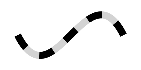
For my work involving canvas I was interested in the implemention of precise dashing of curves. That is to say, given a curve (such as a Bézier curve) we want to place line segments, alternated by spaces, of equal lengths along the curve (see Fig. 1). This means that for a curve parametrized by $t\in[t_0,t_1]$ we want to relate $t$ and $L$, with $L$ the length between $[t_0,t]$. For Béziers we take $t_0=0$ as the start of the curve and $t_1=1$ the end. For elliptical arcs we take $t_0=\theta_{min}$ the start angle and $t_1=\theta_{max}$ the end angle.
Calculating the length of these curves cannot be solved analyticlly, so we will have to approach this numerically. In short, we will approach the integral that gives the length $L$ given a $t$ by Gauss-Legendre quadratures. By picking a couple of points along the curve and obtaining their lengths, we can approximate the real length function $L = s(t)$ as a polynomial by finding a low-degree polynomial $\hat{s}(t)$ that approximates $s(t)$. Given $\hat{s}(t)$ we can easily calculate any length along the curve without taking a big performance hit. I will also show the inverse problem $t = q(L)$ by calculating an appropriate $\hat{q}(L)$ and finally show how Chebyshev approximations can greatly improves our results.
Arc lengths
Given a general parametric curve $C(t) = (x(t), y(t))$, remember that calculating an arc length involves integrating its derivate along the curve, $$ s(t) = \int^{t_1}_{t_0} C’(t) ,dt \tag{1} $$
For example for cubic Béziers we have $$ \begin{align} C(t) &= (1-t)^3P_0 + 3(1-t)^2tP_1 + 3(1-t)t^2P_2 + t^3P_3 \\\ C’(t) &= 3(1-t)^2(P_1-P_0) + 6(1-t)t(P_2-P_1) + 3t^2(P_3-P_2) \end{align} $$ with $P_0$, $P_1$, $P_2$, and $P_3$ the control points. For elliptical arcs we have $$ \begin{align} C(t) &= (a\cos t, b\sin t) \\\ C’(t) &= (-a\sin t, b\cos t) \end{align} $$ with $0 \leq t \leq 2\pi$ and $a$ and $b$ the radii.
As the integral in Eq. 1 cannot be calculated analytically, we will use Gauss-Legendre quadratures to obtain an approximate value for the integral, ie. $$ \int^{t_1}_{t_0} C’(t) dt \approx \frac{t_1-t_0}{2}\sum_{i=1}^n w_iC’\left(\frac{t_1-t_0}{2}x_i+\frac{t_1+t_0}{2}\right)$$ The weights $w_i$ and positions $x_i$ can be obtained from this extensive list for example, but for $n=5$ they are defined as: $$ \begin{array} i &w_i &x_i \\\ \hline 1 &0.5688888888888889 &0.0 \\\ 2 &0.4786286704993665 &-0.5384693101056831 \\\ 3 &0.4786286704993665 &0.5384693101056831 \\\ 4 &0.2369268850561891 &-0.9061798459386640 \\\ 5 &0.2369268850561891 &0.9061798459386640 \\\ \hline \end{array} $$
Length function
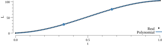
First we want to obtain a function $L = s(t)$ that gives the length $L$ given a parametric value $t$. We will evaluate the curve length at various values of $t$ and from that build a polynomial†. In particular we will find a cubic polynomial $\hat{s}(t)$ that approximates $s(t)$ so that we need to pick four points along the curve. We will pick $t_0=0$, $t_1=\frac{1}{3}$, $t_2=\frac{2}{3}$, $t_3=1$. Note that when $t$ is not in $[0,1]$ we can easily map it to be in that range and later on reverse the mapping (as is needed for elliptical arcs). Now we’d like to find the lengths $L_0$, $L_1$, $L_2$, and $L_3$ corresponding to the $t$’s. $L_0=0$ is easy, for the other three we will use Gauss-Legendre to find their values.
Our polynomial has the form $$\hat{s}(t) = at^3+bt^2+ct+d \tag{2}$$ so that we will concern ourselves with finding the coefficients $a$, $b$, $c$, and $d$. As our length polynomial will go through $(0,0)$ since our first point is at $t_0=0, L_0=0$, the $d$ coefficient is zero and we can drop it out of our equation. The problem then essentially comes down to solving a linear system of three equations. We can express this in matrix form as $$ \begin{bmatrix} L_1 \\\ L_2 \\\ L_3 \\\ \end{bmatrix} = \begin{bmatrix} t_1^3 & t_1^2 & t_1 \\\ t_2^3 & t_2^2 & t_2 \\\ t_3^3 & t_3^2 & t_3 \\\ \end{bmatrix} \begin{bmatrix} a \\\ b \\\ c \\\ \end{bmatrix} = \begin{bmatrix} \frac{1}{27} & \frac{1}{9} & \frac{1}{3} \\\ \frac{8}{27} & \frac{4}{9} & \frac{2}{3} \\\ 1 & 1 & 1 \end{bmatrix} \begin{bmatrix} a \\\ b \\\ c \\\ \end{bmatrix} \tag{3} $$ so that $$ \begin{bmatrix} a \\\ b \\\ c \\\ \end{bmatrix} = \begin{bmatrix} \frac{1}{27} & \frac{1}{9} & \frac{1}{3} \\\ \frac{8}{27} & \frac{4}{9} & \frac{2}{3} \\\ 1 & 1 & 1 \end{bmatrix}^{-1} \begin{bmatrix} L_1 \\\ L_2 \\\ L_3 \\\ \end{bmatrix} = \frac{1}{2} \begin{bmatrix} 27 & -27 & 9 \\\ -45 & 36 & -9 \\\ 18 & -9 & 2 \end{bmatrix} \begin{bmatrix} L_1 \\\ L_2 \\\ L_3 \\\ \end{bmatrix} \tag{4} $$ . This leaves us with calculating $$ \begin{align} a &= 13.5L_1 - 13.5L_2 + 4.5L_3 \\\ b &= -22.5L_1 + 18L_2 - 4.5L_3 \\\ c &= 9.0L_1 - 4.5L_2 + L_3 \\\ \end{align} $$ and filling in those values in our cubic polynomial. See Fig. 2 for and example of a length function on a cubic Bézier.
Inverse length function
Simply inversing the parameters $t$ and $L$ in Eq. 2 would allow us to approximate the inverse problem where we want to known $t$ given an $L$. That is, we’re looking for a polynomial of the form $$\hat{q}(t) = aL^3+bL^2+cL+d$$ which in matrix form is similar to Eq. 3 and 4 and picking $t_1$ at $\frac{1}{3}L_3$, $t_2$ at $\frac{2}{3}L_3$, and $t_3$ at $L_3$ and can be written as $$ \begin{bmatrix} t_1 \\\ t_2 \\\ t_3 \\\ \end{bmatrix} = \begin{bmatrix} L_1^3 & L_1^2 & L_1 \\\ L_2^3 & L_2^2 & L_2 \\\ L_3^3 & L_3^2 & L_3 \\\ \end{bmatrix} \begin{bmatrix} a \\\ b \\\ c \\\ \end{bmatrix} = \begin{bmatrix} \frac{1}{27} & \frac{1}{9} & \frac{1}{3} \\\ \frac{8}{27} & \frac{4}{9} & \frac{2}{3} \\\ 1 & 1 & 1 \end{bmatrix} \begin{bmatrix} aL_3^3 \\\ bL_3^2 \\\ cL_3 \\\ \end{bmatrix} \tag{4} $$ $$ \begin{bmatrix} aL_3^3 \\\ bL_3^2 \\\ cL_3 \\\ \end{bmatrix} = \frac{1}{2} \begin{bmatrix} 27 & -27 & 9 \\\ -45 & 36 & -9 \\\ 18 & -9 & 2 \end{bmatrix} \begin{bmatrix} t_1 \\\ t_2 \\\ t_3 \\\ \end{bmatrix} \tag{5} $$ leading to $$ \begin{align} a &= (13.5t_1 - 13.5t_2 + 4.5t_3) / L_3^3 \\\ b &= (-22.5t_1 + 18t_2 - 4.5t_3) / L_3^2 \\\ c &= (9.0t_1 - 4.5t_2 + t_3) / L_3 \\\ \end{align} $$
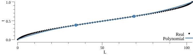
The reason why the $L_i$’s need to be at those intervals is so that we can easily construct a matrix as in Eq. 4 that is easily invertable into Eq. 5. The problem now is finding $t_i$ so that $L_i$ is exactly at equal intervals of $\frac{1}{3}$. This can be done by either first calculating the length function $L = s(t)$ as we did previously, which might be the fastest way to find $t_i$. Another way could be to use the bisection method on the Gauss-Legendre function. This will repeatedly evaluate the length of the curve at various $t$’s until it find $t_i$ that corresponds to $L_i$. First we calculate the total length $L_3$ of the curve using Gauss-Legendre, then we find $t_1$ giving $L_1 = \frac{1}{3}L_3$ by using the bisection method on the interval of $t\in[t_0,t_1]$ and the same for $t_2$ giving $L_2 = \frac{2}{3}L_3$. See Fig. 3 for the inverse length function on a cubic Bézier.
Chebyshev approximation
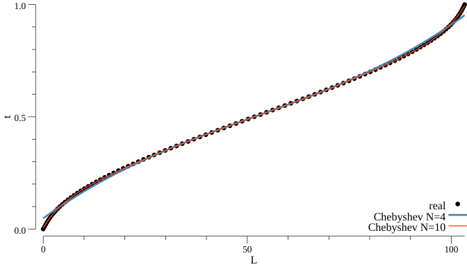
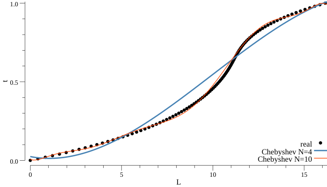
In order to improve the result of Fig. 3, we’ll introduce the use of Chebyshev approximation resulting in a linear combination of Chebyshev polynomials. This will pick better points along the curve which will reduce the errors. Additionally, it is really easy to increase the number of Chebyshev points to increase precision, which is harder with the previously discussed method that needs to invert a matrix. Chebyshev approximates a function $f(x)$ and is defined as $$f(x) \approx -\frac{1}{2}+\sum_{j=0}^{N-1} c_jT_j(x) \\\ T_j(x) = \cos(j\cos^{-1}(x))$$ This is a linear combination of $T_j(x)$ with the $c_j$ coefficients defined on the Chebyshev nodes $$c_j \equiv \frac{2}{N}\sum_{k=1}^Nf(x_k)T_j(x_k) \\\ x_k = \cos\left(\pi\frac{k-\frac{1}{2}}{N}\right) \\\ T_j(x_k) = \cos\left(j\pi\frac{k-\frac{1}{2}}{N}\right) $$ Be aware that $x\in[-1,1]$ and will need to be mapped to the range you want to interpolate $f(x)$.
See Fig. 4 and 5 for the results. With ten Chebyshev nodes we quite accurately approach the data. Choosing a proper $N$ depends on the curve as for some curves a small $N$ might be sufficient but other curves are hard to approximate by a polynomial. The value of $c_j$ is a good indication for the error and it will decrease for increasing $j$. When a number of consecutive $c_j$’s are below a threshold value it is considered accurate enough.
Closing notes
Chebyshev approximation gives good accuracy for most cubic Béziers and elliptical arcs, however you should decide on the magnitude of $N$ yourself as this is highly dependent on the type of curves you want to approximate. If you want to see an implementation in Go, please check path_util.go. It has functions for Gauss-Legendre, the bisection method, the polynomial approximations and the Chebyshev approximation.